Slicing and Tallied BAMs for Interested Genes and Variant Analysis
Peter Huang
Van Andel Institute, Michigan State University13 July 2024
BamSliceR.Bioc2024.RmdAbstract
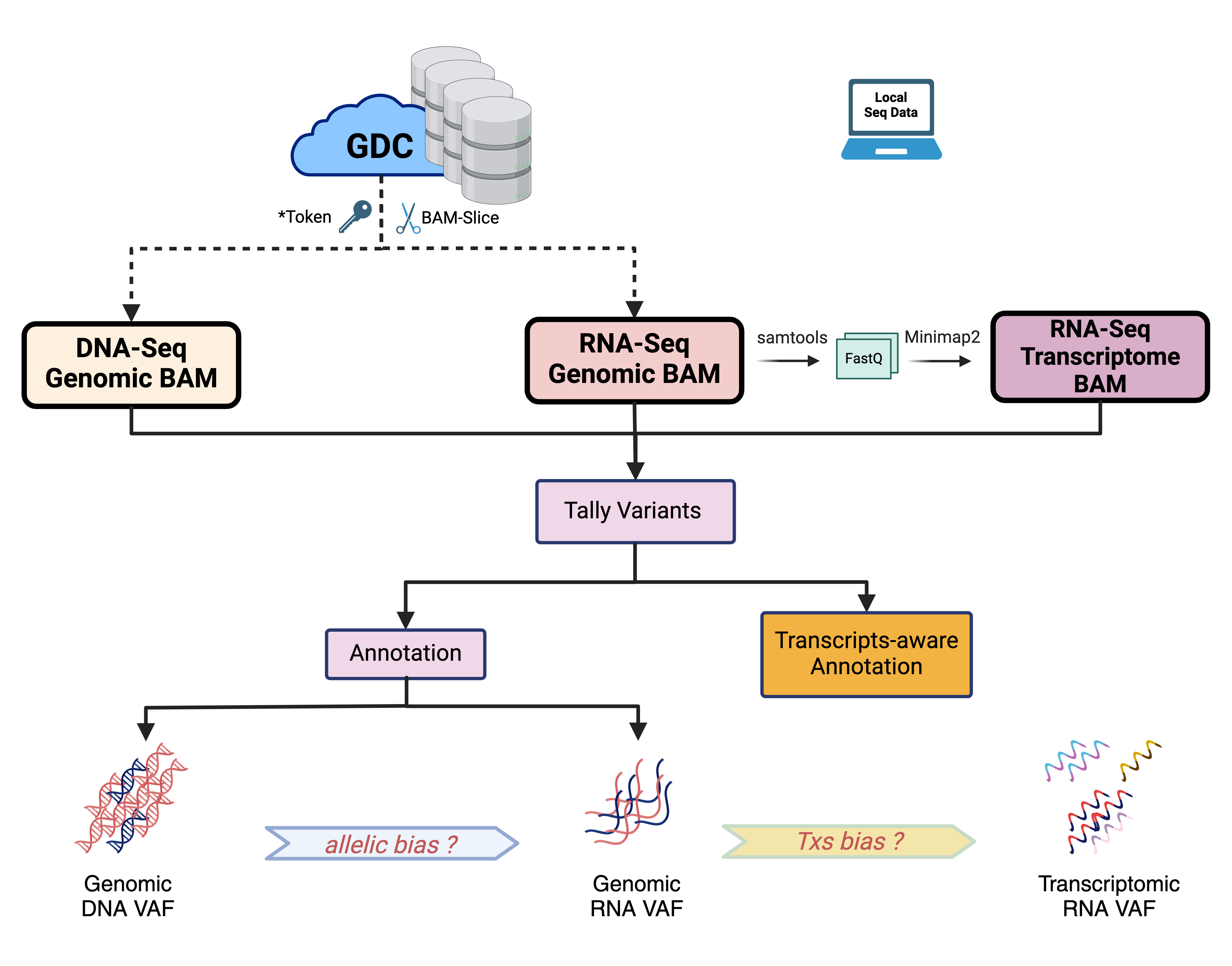
In this vignette, we will walk through the bamSliceR
toolset to swiftly extract coordinate- or range-based aligned DNA and/or
RNA sequence reads from the Genomic Data Commons GDC. We will then demonstrate
the downstream functionality to tally and annotate variants from BAM
files, whether they are stored in the cloud or locally. Also, we want to
highlight the new utilities we implemented in the bamSliceR
to facilitate transcript-aware variants annotation using transcriptome
BAM that generated by aligning reads from RNA-seq to reference
transcripts sequences (GENCODE v36).
We will use data from TARGET (Bolouri et al., 2017), BEAT-AML (Tyner et al., 2018) and Leucegene (Lavallée et al., 2016).
Introduction
We developed bamSliceR to address two practical
challenges: resource-sparing identification of candidate subjects, and
variant detection from aligned sequence reads across thousands of
controlled-access subjects. The GDC (Wilson et al., 2017) BAM
Slicing API is a practical and well-documented REST API for this
purpose. (Morgan and
Davis, 2017). Additionally, the
GenomicDataCommons Bioconductor package implements the
service in R interface, allowing for more efficient querying of data
from the GDC. However, we find relatively little published work that
uses the GDC API, even those evaluating specific candidate variants.
Instead, researchers often rely on variant calls from previous studies,
assuming a single best method for variant detection fits all
experimental designs—a notion contradicted by various benchmarks.
Alternatively, retrieving and reanalyze raw sequence data, which is
highly inefficient.
bamSliceR pipeline
* If you will be analyzing any data that is controlled access, you will need to download a GDC token and store it in a file in your home directory. For more instructions see GenomicDataCommons Token and Data portal authentication tokens
Working with Genomic BAM files
Download Bam Slices
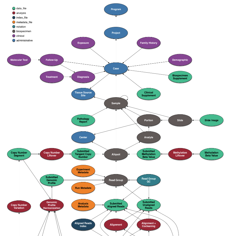
The data model for the GDC is complex. If you want query more other types of data, it may worth to overview the details. Here, we focus on identifying the metadata of BAM files, followed by downloading the sliced BAM.
Identify the BAM file of interest
We simplified the querying process in a single function to gather BAM files information from the project of interest.
file_meta = getGDCBAMs(projectId = "TARGET-AML",
                       es = "RNA-Seq",
                       workflow = "STAR 2-Pass Genome")
nrow(file_meta)
## [1] 3225
head(file_meta)## id sample
## 1 7d4d460b-5ac9-4a6f-83f8-b25f22c5dcad TARGET-20-PASNKC-09A-01R
## 2 33194131-ddc9-417a-ab6d-22c01acc6c7d TARGET-20-PASNLR-03A-01R
## 3 c2e1548b-e75f-435a-9228-a3cbf9dfd051 TARGET-20-PASNAL-09A-01R
## 4 e68b2f1b-fcc4-4a28-8505-bc88e15551a5 TARGET-20-PASNDA-09A-01R
## 5 4d636562-b5fd-4bdf-b3eb-067210786f34 TARGET-20-PATLIG-09A-02R
## 6 794532f5-c57e-4fec-a9dd-fb3e3a5e936d TARGET-20-PASNYB-09A-01R
## file_name case_id
## 1 4437f783-96e7-43a8-87ef-5fed5b4c91ab.rna_seq.genomic.gdc_realn.bam TARGET-20-PASNKC
## 2 84bba567-4acc-4ee6-8f19-e15b7a87ed08.rna_seq.genomic.gdc_realn.bam TARGET-20-PASNLR
## 3 039a1e3a-b7b6-4bc8-8c52-1c7f82cbaa62.rna_seq.genomic.gdc_realn.bam TARGET-20-PASNAL
## 4 5887ccad-c7a4-454a-9c50-d223bb144c78.rna_seq.genomic.gdc_realn.bam TARGET-20-PASNDA
## 5 e8bbcbd2-1cc1-41be-89b7-032264703bf6.rna_seq.genomic.gdc_realn.bam TARGET-20-PATLIG
## 6 e0a2b8e3-f8fb-480c-96e6-bfca08f09934.rna_seq.genomic.gdc_realn.bam TARGET-20-PASNYB
## sample_type experimental_strategy
## 1 Primary Blood Derived Cancer - Bone Marrow RNA-Seq
## 2 Primary Blood Derived Cancer - Peripheral Blood RNA-Seq
## 3 Primary Blood Derived Cancer - Bone Marrow RNA-Seq
## 4 Primary Blood Derived Cancer - Bone Marrow RNA-Seq
## 5 Primary Blood Derived Cancer - Bone Marrow RNA-Seq
## 6 Primary Blood Derived Cancer - Bone Marrow RNA-Seq
## workflow
## 1 STAR 2-Pass Genome
## 2 STAR 2-Pass Genome
## 3 STAR 2-Pass Genome
## 4 STAR 2-Pass Genome
## 5 STAR 2-Pass Genome
## 6 STAR 2-Pass Genome
## downloaded_file_name
## 1 TARGET-20-PASNKC-09A-01R_TARGET-20-PASNKC_4437f783-96e7-43a8-87ef-5fed5b4c91ab.rna_seq.genomic.gdc_realn.bam
## 2 TARGET-20-PASNLR-03A-01R_TARGET-20-PASNLR_84bba567-4acc-4ee6-8f19-e15b7a87ed08.rna_seq.genomic.gdc_realn.bam
## 3 TARGET-20-PASNAL-09A-01R_TARGET-20-PASNAL_039a1e3a-b7b6-4bc8-8c52-1c7f82cbaa62.rna_seq.genomic.gdc_realn.bam
## 4 TARGET-20-PASNDA-09A-01R_TARGET-20-PASNDA_5887ccad-c7a4-454a-9c50-d223bb144c78.rna_seq.genomic.gdc_realn.bam
## 5 TARGET-20-PATLIG-09A-02R_TARGET-20-PATLIG_e8bbcbd2-1cc1-41be-89b7-032264703bf6.rna_seq.genomic.gdc_realn.bam
## 6 TARGET-20-PASNYB-09A-01R_TARGET-20-PASNYB_e0a2b8e3-f8fb-480c-96e6-bfca08f09934.rna_seq.genomic.gdc_realn.bam
## UPC_ID
## 1 PASNKC
## 2 PASNLR
## 3 PASNAL
## 4 PASNDA
## 5 PATLIG
## 6 PASNYBThree pieces of information are needed to locate the BAM files on GDC
portal, which can be inspected by availableProjectId(),
availableExpStrategy() and
availableWorkFlow(), respectively.
- The project ID.
- Experiment Strategy (ex. “RAN-Seq”, “WGS”, etc. )
- Alignment workflow.
availableProjectId() %>% head(n = 10)## [1] "HCMI-CMDC" "TCGA-BRCA" "TARGET-ALL-P3"
## [4] "EXCEPTIONAL_RESPONDERS-ER" "CGCI-HTMCP-LC" "CPTAC-2"
## [7] "CMI-MBC" "TARGET-ALL-P2" "OHSU-CNL"
## [10] "TARGET-ALL-P1"
availableExpStrategy("TARGET-AML")## [1] "Genotyping Array" "Methylation Array" "RNA-Seq"
## [4] "Targeted Sequencing" "WGS" "WXS"
## [7] "miRNA-Seq"
availableWorkFlow(projectId = "TARGET-AML", es = "RNA-Seq")## doc_count key
## 1 6450 Arriba
## 2 6450 STAR - Counts
## 3 6450 STAR-Fusion
## 4 3225 STAR 2-Pass Chimeric
## 5 3225 STAR 2-Pass Genome
## 6 3225 STAR 2-Pass TranscriptomeIdentify the Genomic Ranges of interest
BAM slicing API from GDC portal accept genomic ranges specifying as vector of character() e.g., c(“chr”, “chr1:10000”). Here we provide a function to get the required input format given the gene names.
target_genes_data = system.file("extdata", "gene_names.rds", package = "bamSliceR")
target_genes = readRDS(target_genes_data)
target_genes
## IDH1 IDH2 TET1 TET2 ASXL1 ASXL2 DNMT3A RUNX1 HIST1H3A HIST1H3B
## "IDH1" "IDH2" "TET1" "TET2" "ASXL1" "ASXL2" "DNMT3A" "RUNX1" "H3C1" "H3C2"
## HIST1H3C HIST1H3D HIST1H3E HIST1H3F HIST1H3G HIST1H3H HIST1H3I HIST1H3J H3F3A
## "H3C3" "H3C4" "H3C6" "H3C7" "H3C8" "H3C10" "H3C11" "H3C12" "H3-3A"Get either GRanges or vector of character()
for exons of the genes.
#Get GRanges for exons of all genes above
target_ranges_gr = getGenesCoordinates(target_genes, ret = "GRanges")
head(target_ranges_gr)
## GRanges object with 6 ranges and 0 metadata columns:
## seqnames ranges strand
## <Rle> <IRanges> <Rle>
## ASXL1 20 32358280-32439369 +
## ASXL2 2 25733703-25878537 -
## DNMT3A 2 25227805-25342640 -
## H3-3A 1 226061801-226072069 +
## H3C1 6 26020401-26021008 +
## H3C10 6 27810001-27811350 +
## -------
## seqinfo: 8 sequences from an unspecified genome; no seqlengths
#Get the vector of character() instead.
target_ranges_chars = getGenesCoordinates(target_genes, ret ="DF",
                                          extendEnds = 100)
head(target_ranges_chars)
## [1] "chr20:32358230-32439419" "chr2:25733653-25878587" "chr2:25227755-25342690"
## [4] "chr1:226061751-226072119" "chr6:26020351-26021058" "chr6:27809951-27811400"Download sliced-BAM
downloadSlicedBAMs(file_df = file_meta,
                   regions = target_ranges_chars,
                   dir = "BAM_FILES")
Tally Variants from sliced BAMs
bamSliceR integrated functionality in Bioconductor
package gmapR (gmapR) to tally coverage and
counts of variant alleles followed by estimation of Variant Allele
Fraction (VAF) of each variants.
Identify the Genomic Ranges of interest
We first also need to specify the regions as a GRanges
object, which can be a subset of genomic ranges used to sliced BAM
files.
head(target_ranges_gr)## GRanges object with 6 ranges and 0 metadata columns:
## seqnames ranges strand
## <Rle> <IRanges> <Rle>
## ASXL1 20 32358280-32439369 +
## ASXL2 2 25733703-25878537 -
## DNMT3A 2 25227805-25342640 -
## H3-3A 1 226061801-226072069 +
## H3C1 6 26020401-26021008 +
## H3C10 6 27810001-27811350 +
## -------
## seqinfo: 8 sequences from an unspecified genome; no seqlengthsSpecify list of BAM files
Then we need make a text file to include all the names of downloaded BAM files.
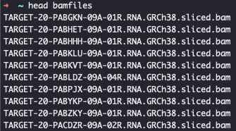
Terminal command
In the directory of the downloaded BAM files, we then
scan the ‘bamfiles’ into R.
bamfiles_txt = system.file("extdata", "bamfiles", package = "bamSliceR")
bamfiles = scan(bamfiles_txt, "character")
Preparing gmapGenome Object
Last thing we need is to create a gmapGenome object,
then specify the directory of it.
#GmapGenome objects can be created from FASTA files or BSgenome objects. Below is
#an example of how to create human hg38 gmapGenome from BSgenome.

library(gmapR)
library(BSgenome.Hsapiens.UCSC.hg38)

gmapGenomePath <- file.path("PATH/to/SAVE/gmapGenome", "hg38")
gmapGenomeDirectory <- GmapGenomeDirectory(gmapGenomePath, create = TRUE)

gmapGenome <- GmapGenome(genome=Hsapiens,
                         directory=gmapGenomeDirectory,
                         name="hg38", create=TRUE)
Tallying Reads
We can then start to tally the reads of BAM files. If you want to run
tallyReads on machine with multiple nodes, there are
parameters to distribute the nodes according to number of BAM files and
number of genomic ranges:
-
parallelOnRanges: ifTRUE, will process the Genomic Ranges in parallel. -
parallelOnRangesBPPARAM: configuration for parallel tallyreads on genomic ranges. -
BPPARAM: configuration for parallel tallyreads on BAM files.
If we want to tally reads on thousands of BAM but only few gene regions, ideally we want to put more workers on computing on BAM files but less workers on granges regions.
tallied_reads = tallyReads(bamfiles = bamfiles, gmapGenome_dir = gmapGenome_dir,
                           grs = target_ranges,
                           BPPARAM = MulticoreParam(workers = 4 , stop.on.error = TRUE),
                           parallelOnRanges = TRUE,
                           parallelOnRangesBPPARAM = MulticoreParam(workers = 4) )
We also provide a bash template
to run tallyReads() on HPC on large cohorts.
Annotation of Variants tallied from Genomic BAM files
Annotation of Variants
A VRanges object will be generated from tallying reads
from BAM files, contains all the putative variants.
sampleNames() can be used to see the name of BAM files
which variants detected from. Here, We present an example on how to
annotate variants with predicted consequence using VariantAnnotation
and Ensembl Variant Effect Predictor (VEP).
We started from a VRanges output from
tallyReads().
library(bamSliceR)
tallied_reads = system.file("extdata", "tallied_reads_example.rds",
                            package = "bamSliceR")
tallied_reads_vr = readRDS(tallied_reads)
tallied_reads_vr[4565:4566]
## VRanges object with 2 ranges and 17 metadata columns:
## seqnames ranges strand ref alt totalDepth
## <Rle> <IRanges> <Rle> <character> <characterOrRle> <integerOrRle>
## [1] chr1 226066383 * A G 139
## [2] chr1 226066384 * T C 96
## refDepth altDepth sampleNames softFilterMatrix | n.read.pos
## <integerOrRle> <integerOrRle> <factorOrRle> <matrix> | <integer>
## [1] 138 1 TARGET-20-PAVLZE-09A.. | 1
## [2] 95 1 TARGET-20-PAVHCV-09A.. | 1
## n.read.pos.ref raw.count.total count.plus count.plus.ref count.minus
## <integer> <integer> <integer> <integer> <integer>
## [1] 60 139 1 90 0
## [2] 49 96 1 65 0
## count.minus.ref count.del.plus count.del.minus read.pos.mean read.pos.mean.ref
## <integer> <integer> <integer> <numeric> <numeric>
## [1] 48 0 0 67 33.0652
## [2] 30 0 0 35 31.8316
## read.pos.var read.pos.var.ref mdfne mdfne.ref count.high.nm count.high.nm.ref
## <numeric> <numeric> <numeric> <numeric> <integer> <integer>
## [1] NA 420.538 NA NA 1 138
## [2] NA 479.346 NA NA 1 95
## -------
## seqinfo: 2779 sequences (1 circular) from 2 genomes (hg38, NA)
## hardFilters: NULL
# VRanges-specific methods such as altDepth(), refDepth(), totalDepth() would not
# availiable after conversion to GRanges. So save those info now.
tallied_reads_vr = saveVRinfo(tallied_reads_vr)
tallied_reads_vr[4565:4566]
## VRanges object with 2 ranges and 23 metadata columns:
## seqnames ranges strand ref alt totalDepth
## <Rle> <IRanges> <Rle> <character> <characterOrRle> <integerOrRle>
## [1] chr1 226066383 * A G 139
## [2] chr1 226066384 * T C 96
## refDepth altDepth sampleNames softFilterMatrix | n.read.pos
## <integerOrRle> <integerOrRle> <factorOrRle> <matrix> | <integer>
## [1] 138 1 TARGET-20-PAVLZE-09A.. | 1
## [2] 95 1 TARGET-20-PAVHCV-09A.. | 1
## n.read.pos.ref raw.count.total count.plus count.plus.ref count.minus
## <integer> <integer> <integer> <integer> <integer>
## [1] 60 139 1 90 0
## [2] 49 96 1 65 0
## count.minus.ref count.del.plus count.del.minus read.pos.mean read.pos.mean.ref
## <integer> <integer> <integer> <numeric> <numeric>
## [1] 48 0 0 67 33.0652
## [2] 30 0 0 35 31.8316
## read.pos.var read.pos.var.ref mdfne mdfne.ref count.high.nm count.high.nm.ref
## <numeric> <numeric> <numeric> <numeric> <integer> <integer>
## [1] NA 420.538 NA NA 1 138
## [2] NA 479.346 NA NA 1 95
## ref alt totalDepth refDepth altDepth VAF
## <character> <character> <integer> <integer> <integer> <numeric>
## [1] A G 139 138 1 0.00719424
## [2] T C 96 95 1 0.01041667
## -------
## seqinfo: 2779 sequences (1 circular) from 2 genomes (hg38, NA)
## hardFilters: NULL
# Match back the metadata of BAM files to the VRanges
#file_meta = getGDCBAMs("TARGET-AML", "RNA-Seq", "STAR 2-Pass Genome")
tallied_reads_vrinfo_baminfo = annotateWithBAMinfo(tallied_reads_vr, file_meta)
tallied_reads_vrinfo_baminfo[4565:4566]
## VRanges object with 2 ranges and 32 metadata columns:
## seqnames ranges strand ref alt totalDepth
## <Rle> <IRanges> <Rle> <character> <characterOrRle> <integerOrRle>
## [1] chr1 226066383 * A G 139
## [2] chr1 226066384 * T C 96
## refDepth altDepth sampleNames softFilterMatrix | n.read.pos
## <integerOrRle> <integerOrRle> <factorOrRle> <matrix> | <integer>
## [1] 138 1 TARGET-20-PAVLZE-09A.. | 1
## [2] 95 1 TARGET-20-PAVHCV-09A.. | 1
## n.read.pos.ref raw.count.total count.plus count.plus.ref count.minus
## <integer> <integer> <integer> <integer> <integer>
## [1] 60 139 1 90 0
## [2] 49 96 1 65 0
## count.minus.ref count.del.plus count.del.minus read.pos.mean read.pos.mean.ref
## <integer> <integer> <integer> <numeric> <numeric>
## [1] 48 0 0 67 33.0652
## [2] 30 0 0 35 31.8316
## read.pos.var read.pos.var.ref mdfne mdfne.ref count.high.nm count.high.nm.ref
## <numeric> <numeric> <numeric> <numeric> <integer> <integer>
## [1] NA 420.538 NA NA 1 138
## [2] NA 479.346 NA NA 1 95
## ref alt totalDepth refDepth altDepth VAF
## <character> <character> <integer> <integer> <integer> <numeric>
## [1] A G 139 138 1 0.00719424
## [2] T C 96 95 1 0.01041667
## id sample file_name
## <character> <character> <character>
## [1] 6cb02b4d-ca87-4d9d-a.. TARGET-20-PAVLZE-09A.. 09b91534-5759-4000-9..
## [2] f74f1d3f-8774-4bd2-b.. TARGET-20-PAVHCV-09A.. 6b5b7906-4220-4f7d-b..
## case_id sample_type experimental_strategy workflow
## <character> <character> <character> <character>
## [1] TARGET-20-PAVLZE Primary Blood Derive.. RNA-Seq STAR 2-Pass Genome
## [2] TARGET-20-PAVHCV Primary Blood Derive.. RNA-Seq STAR 2-Pass Genome
## downloaded_file_name UPC_ID
## <character> <character>
## [1] TARGET-20-PAVLZE-09A.. PAVLZE
## [2] TARGET-20-PAVHCV-09A.. PAVHCV
## -------
## seqinfo: 2779 sequences (1 circular) from 2 genomes (hg38, NA)
## hardFilters: NULL
# Only keep variants with variant allele frequency greater than 5%.
tallied_reads_vrinfo_baminfo = subset(tallied_reads_vrinfo_baminfo, VAF > 0.05)
VariantAnnotation
Consequence of variants now can be predicted using VariantAnnotation:
getVariantAnnotation(tallied_reads_vrinfo_baminfo) -> tallied_reads_vrinfo_baminfo_gr
tallied_reads_vrinfo_baminfo_gr[,c("UPC_ID", bamSliceR:::.VARIANT_ANNOTATE_INFO)]
## GRanges object with 55017 ranges and 15 metadata columns:
## seqnames ranges strand | UPC_ID varAllele CDSLOC
## <Rle> <IRanges> <Rle> | <character> <DNAStringSet> <IRanges>
## [1] chr1 143905605 - | PAVCJW G 189
## [2] chr1 143905605 - | PAVCJW G 362
## [3] chr1 143905634 - | PAVHLI A 160
## [4] chr1 143905634 - | PAVHLI A 333
## [5] chr1 143905660 - | PAVDAB A 134
## ... ... ... ... . ... ... ...
## [55013] chr21 34892962 - | PATLFJ AA 60
## [55014] chr21 35048867 - | PASHWN TT 33
## [55015] chr21 35048867 - | PASHWN TT 33
## [55016] chr21 35048881-35048882 - | PAURVI T 18-19
## [55017] chr21 35048881-35048882 - | PAURVI T 18-19
## PROTEINLOC QUERYID TXID CDSID GENEID CONSEQUENCE
## <IntegerList> <integer> <character> <IntegerList> <character> <factor>
## [1] 63 71 17544 21002,21003 440686 nonsynonymous
## [2] 121 71 17545 21002,21003 440686 nonsynonymous
## [3] 54 72 17544 21002,21003 440686 nonsynonymous
## [4] 111 72 17545 21002,21003 440686 nonsense
## [5] 45 73 17544 21002,21003 440686 nonsynonymous
## ... ... ... ... ... ... ...
## [55013] 20 43534 237682 261221 101928269 frameshift
## [55014] 11 43535 237671 261222 861 frameshift
## [55015] 11 43535 237682 261222 101928269 frameshift
## [55016] 6,7 43536 237671 261222 861 frameshift
## [55017] 6,7 43536 237682 261222 101928269 frameshift
## REFCODON VARCODON REFAA VARAA POS CHANGE
## <DNAStringSet> <DNAStringSet> <AAStringSet> <AAStringSet> <integer> <character>
## [1] CAT CAG H Q 63 H63Q
## [2] ATG AGG M R 121 M121R
## [3] CGC AGC R S 54 R54S
## [4] TGC TGA C * 111 C111*
## [5] GGG GAG G E 45 G45E
## ... ... ... ... ... ... ...
## [55013] GAA GAAA 20 20
## [55014] CCT CCTT 11 11
## [55015] CCT CCTT 11 11
## [55016] ATATTT ATTTT 6 6
## [55017] ATATTT ATTTT 6 6
## -------
## seqinfo: 24 sequences from hg38 genomeEnsembl Variant Effect Predictor (VEP)
Consequence of variants also can be predicted using Variant Effect Predictor (VEP). The code below shows how to generate VCF file as input for VEP:
gr2vrforVEP(tallied_reads_vrinfo_baminfo, file = "~/INPUT_VCF_FILE.vcf",
            writeToVcf = TRUE) -> vr

head(vr)
## VRanges object with 6 ranges and 1 metadata column:
## seqnames ranges strand ref alt totalDepth
## <Rle> <IRanges> <Rle> <character> <characterOrRle> <integerOrRle>
## [1] chr1 143894587 * C A 2
## [2] chr1 143894592 * A G 2
## [3] chr1 143894604 * G T 1
## [4] chr1 143894701 * A C 8
## [5] chr1 143894711 * G A 1
## [6] chr1 143894815 * A T 2
## refDepth altDepth sampleNames softFilterMatrix | index
## <integerOrRle> <integerOrRle> <factorOrRle> <matrix> | <character>
## [1] 1 1 VEP | chr1:143894587_C/A
## [2] 1 1 VEP | chr1:143894592_A/G
## [3] 0 1 VEP | chr1:143894604_G/T
## [4] 7 1 VEP | chr1:143894701_A/C
## [5] 0 1 VEP | chr1:143894711_G/A
## [6] 1 1 VEP | chr1:143894815_A/T
## -------
## seqinfo: 2779 sequences from an unspecified genome; no seqlengths
## hardFilters: NULLDetails about how to run Variant Effect Predictor can be found in (ensemblVEP) or (VEP).
The VCF file with variant effect predicted can be annotated back to patients’ variants.
#Example vcf file with variant effect predicted.
# Output VCF file from VEP
vep_file = system.file("extdata", "TARGET_AML_VRforVEP_vep.vcf", package = "bamSliceR")

#Extract the predicted consequences of variants from VEP
csqFromVEP = getCSQfromVEP(vep_file)
head(csqFromVEP)

#Annotated the variants with VEP predicted consequences
tallied_reads_vrinfo_baminfo_annotated_gr = getVEPAnnotation(tallied_reads_vrinfo_baminfo_gr,
                                                             csqFromVEP)
tallied_reads_vrinfo_baminfo_annotated_gr[1523:1525,-c(1:17)]
Missing Reference Read Counts for INDELs in
tallyreads()
indels = subset(tallied_reads_vrinfo_baminfo_annotated_gr,
                bamSliceR:::getVarType(tallied_reads_vrinfo_baminfo_annotated_gr) != "SNP")
summary(indels$VAF)
summary(indels$refDepth)
bamSliceR has a function
fixIndelRefCounts() pileup the total read depth for these
INDELs.
Visualization
To facilitate downstream analysis of variants from patients,
bamSliceR provides customized plotVAF() function based on
the maftools::plotVaF() from maftools
to help user to investigate the Variant Allele Frequency of the selected
variants.
Distribution of VAF
By default, the plotVAF would plot the distribution of
VAF in top genes.
library(bamSliceR)

TARGET_AML_RNA_annotated_file = system.file("extdata", "TARGET_AML_RNA_annotated.gr.rds",
                            package = "bamSliceR")

tallied_reads_vrinfo_baminfo_annotated_gr = readRDS(TARGET_AML_RNA_annotated_file)
plotVAF(tallied_reads_vrinfo_baminfo_annotated_gr, title = "Default: VAF of Top genes")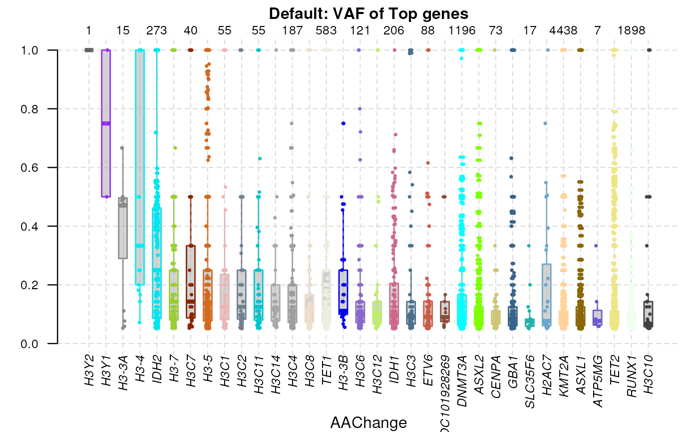
By specifying single gene and multiple coordinates against the gene
products, the plotVAF() would plot distribution of VAF in
selected loci of the gene.
plotVAF(tallied_reads_vrinfo_baminfo_annotated_gr, genes = "IDH2",
        bySingleLocus = c(140, 172), title = "VAF of IDH2 at R140 and R172")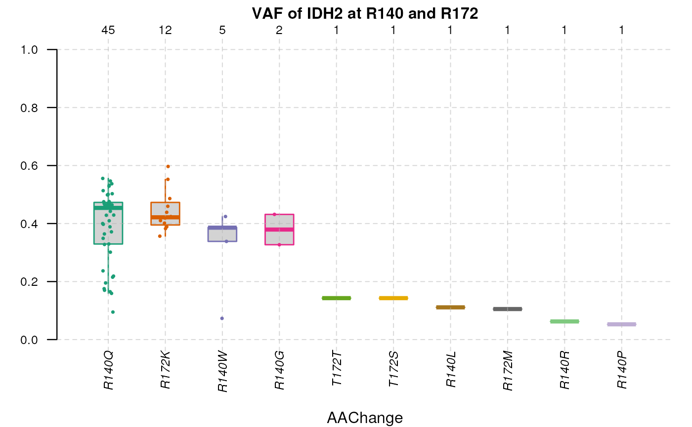
By specifying multiple genes and single coordinate against the genes’
products, the plotVAF() would plot distribution of VAF in
selected loci of the gene.
histone_genes <- c(
  HIST1H3A = "H3C1",
  HIST1H3B = "H3C2",
  HIST1H3C = "H3C3",
  HIST1H3D = "H3C4",
  HIST1H3E = "H3C6",
  HIST1H3F = "H3C7",
  HIST1H3G = "H3C8",
  HIST1H3H = "H3C10",
  HIST1H3I = "H3C11",
  HIST1H3J = "H3C12", H3F3A = "H3-3A"
)

plotVAF (tallied_reads_vrinfo_baminfo_annotated_gr,
         genes = histone_genes,
         bySingleLocus = c(28), title = "VAF of Histone 3 genes at K27")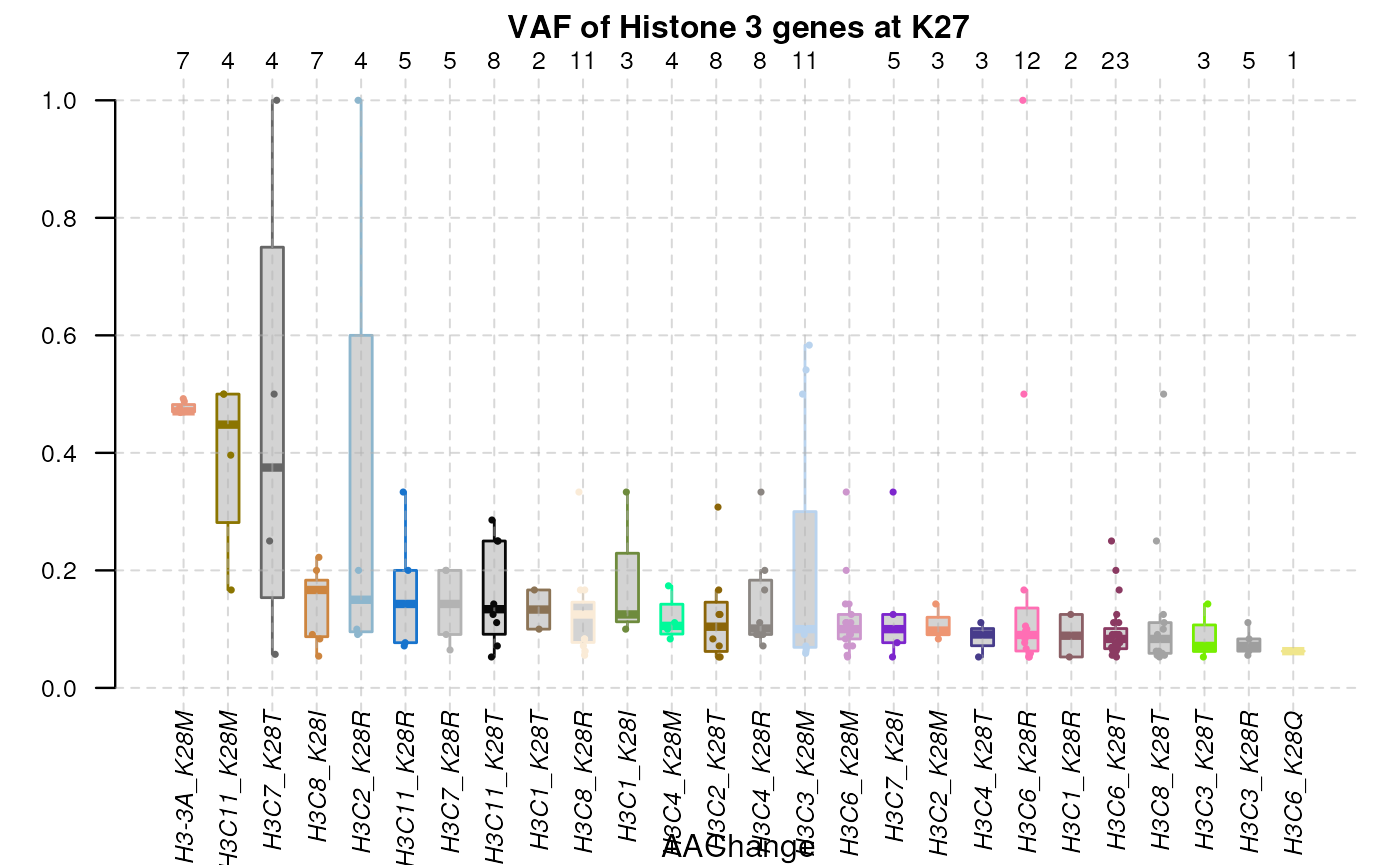
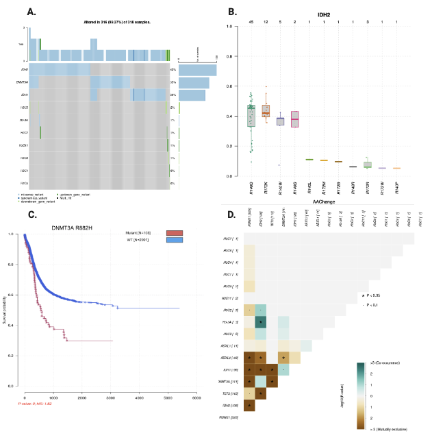
Covert to MAF file format
Also, bamSliceR provides utility that allow conversion
of GRanges to MAF format file, which is
compatible with maftools. Oncoplots, survival analysis, and
mutual exclusive test, etc, can then be implemented easily. More details
in here.
Working with Transcriptome BAM files
![]()
Why Transcriptome BAM ?
Understanding the transcript architecture of genes is crucial for annotating variants determined by raw read counts from RNA-sequencing data. Overlooking or biasing the transcript-specific context may lead to the misinterpretation of the disease-associated effects of these variants.
We implemented in the bamSliceR to facilitate
transcript-aware variants annotation using transcriptome BAM that
generated by aligning reads from RNA-seq to reference transcripts
sequences (GENCODE v36)[https://www.gencodegenes.org/human/release_36.html].
library(rtracklayer)
library(bamSliceR)

leu.file = system.file("extdata", "leucegene.txs.tallied.reads.rds", package = "bamSliceR")
leu.tallied.reads = readRDS(leu.file)
leu.tallied.reads[,c("UPC_ID")] %>% head()
## VRanges object with 6 ranges and 1 metadata column:
## seqnames ranges strand ref alt totalDepth
## <Rle> <IRanges> <Rle> <character> <characterOrRle> <integerOrRle>
## [1] ENST00000366816.5 536-537 * CA C 4
## [2] ENST00000366816.5 578 * C CT 20
## [3] ENST00000366816.5 654 * C CT 11
## [4] ENST00000366816.5 774 * A G 377
## [5] ENST00000366814.3 20 * A C 118
## [6] ENST00000366814.3 97 * G GGGTA 13
## refDepth altDepth sampleNames softFilterMatrix | UPC_ID
## <integerOrRle> <integerOrRle> <factorOrRle> <matrix> | <character>
## [1] 0 4 02H053.RNAseq.gencod.. | 02H053
## [2] 0 20 02H053.RNAseq.gencod.. | 02H053
## [3] 0 11 02H053.RNAseq.gencod.. | 02H053
## [4] 355 19 02H053.RNAseq.gencod.. | 02H053
## [5] 112 6 02H053.RNAseq.gencod.. | 02H053
## [6] 0 13 02H053.RNAseq.gencod.. | 02H053
## -------
## seqinfo: 128 sequences from gencode.v36.txs genome
## hardFilters: NULLAnnotation of Variants tallied from Genomic BAM files
Generate Trancriptomic GENCODE annotation GFF file
Transcriptome BAM files lack the information of genomic coordinates when mapping reads to reference transcripts sequences. Convention GFF3 files, from GENCODE for example, contains the gene annotation on the reference chromosomes, which are not compatible with Transcriptome BAM.
library(rtracklayer)
library(bamSliceR)
coords.column.names = c("seqid", "type", "start", "end", "gene_name")

gencode.v36.file = system.file("extdata", "gencode.v36.annotation.subset.gff3",
                             package = "bamSliceR")
gencode.v36.df = readGFF(gencode.v36.file)
gencode.v36.df[,coords.column.names]
## DataFrame with 2403 rows and 5 columns
## seqid type start end gene_name
## <factor> <factor> <integer> <integer> <character>
## 1 chr1 gene 226061851 226072019 H3-3A
## 2 chr1 transcript 226061851 226071523 H3-3A
## 3 chr1 exon 226061851 226062094 H3-3A
## 4 chr1 exon 226062735 226062811 H3-3A
## 5 chr1 exon 226064329 226064479 H3-3A
## ... ... ... ... ... ...
## 2399 chr21 transcript 35954660 35984749 RUNX1
## 2400 chr21 exon 35984572 35984749 RUNX1
## 2401 chr21 exon 35981751 35981916 RUNX1
## 2402 chr21 exon 35970075 35970167 RUNX1
## 2403 chr21 exon 35954660 35954825 RUNX1In order to easily annotate the tallied variants from transcriptome
BAM, we provide get_txs_coords_of_gff() to calculate the
coordinates of transcripts for each features entity (except “gene”
feature), based on the given genomic coordinates. The function would
maintain the internal structure of the GFF3 file (for example, the
hierarchy of the features for each genes.)
genomic.column.names = c("g_seqid", "g_start", "g_end")
get_txs_coords_of_gff( gencode.file = gencode.v36.file, isSaveGenomicCoords = TRUE) -> gencode.v36.transcripts.df
## [1] "Get index of all feature types in GFF file..."
## [1] "Get the info of each features..."
## [1] "Get the coordinates aginst transcripts..."
## [1] "Swap genomic coordinates with transcripts coordiantes..."
gencode.v36.transcripts.df[,c(coords.column.names, genomic.column.names)]## DataFrame with 2403 rows and 8 columns
## seqid type start end gene_name g_seqid g_start
## <character> <factor> <numeric> <numeric> <character> <factor> <integer>
## 1 chr1 gene 226061851 226072019 H3-3A chr1 226061851
## 2 ENST00000366816.5 transcript 1 799 H3-3A chr1 226061851
## 3 ENST00000366816.5 exon 1 244 H3-3A chr1 226061851
## 4 ENST00000366816.5 exon 245 321 H3-3A chr1 226062735
## 5 ENST00000366816.5 exon 322 472 H3-3A chr1 226064329
## ... ... ... ... ... ... ... ...
## 2399 ENST00000460207.1 transcript 1 603 RUNX1 chr21 35954660
## 2400 ENST00000460207.1 exon 1 178 RUNX1 chr21 35984572
## 2401 ENST00000460207.1 exon 179 344 RUNX1 chr21 35981751
## 2402 ENST00000460207.1 exon 345 437 RUNX1 chr21 35970075
## 2403 ENST00000460207.1 exon 438 603 RUNX1 chr21 35954660
## g_end
## <integer>
## 1 226072019
## 2 226071523
## 3 226062094
## 4 226062811
## 5 226064479
## ... ...
## 2399 35984749
## 2400 35984749
## 2401 35981916
## 2402 35970167
## 2403 35954825Find all Transcripts of Gene Compatible with a Variant
Transcripts that overlap with a variant but have few or no reads mapped to them may not be recorded or could be filtered out. However, these cases are still informative for addressing questions such as why mutated transcripts are not expressed, and whether the mutation triggers mechanisms like nonsense-mediated decay that eliminate the mutated transcripts. In this case, we want to re-tally reads for these transcripts that compatible with the variant.
For each genes, bamSliceR has function
getDisjoinOverlapBins to create disjoint bins that each bin
contains the information of both transcriptome and genomic coordinates
of overlapped transcripts. 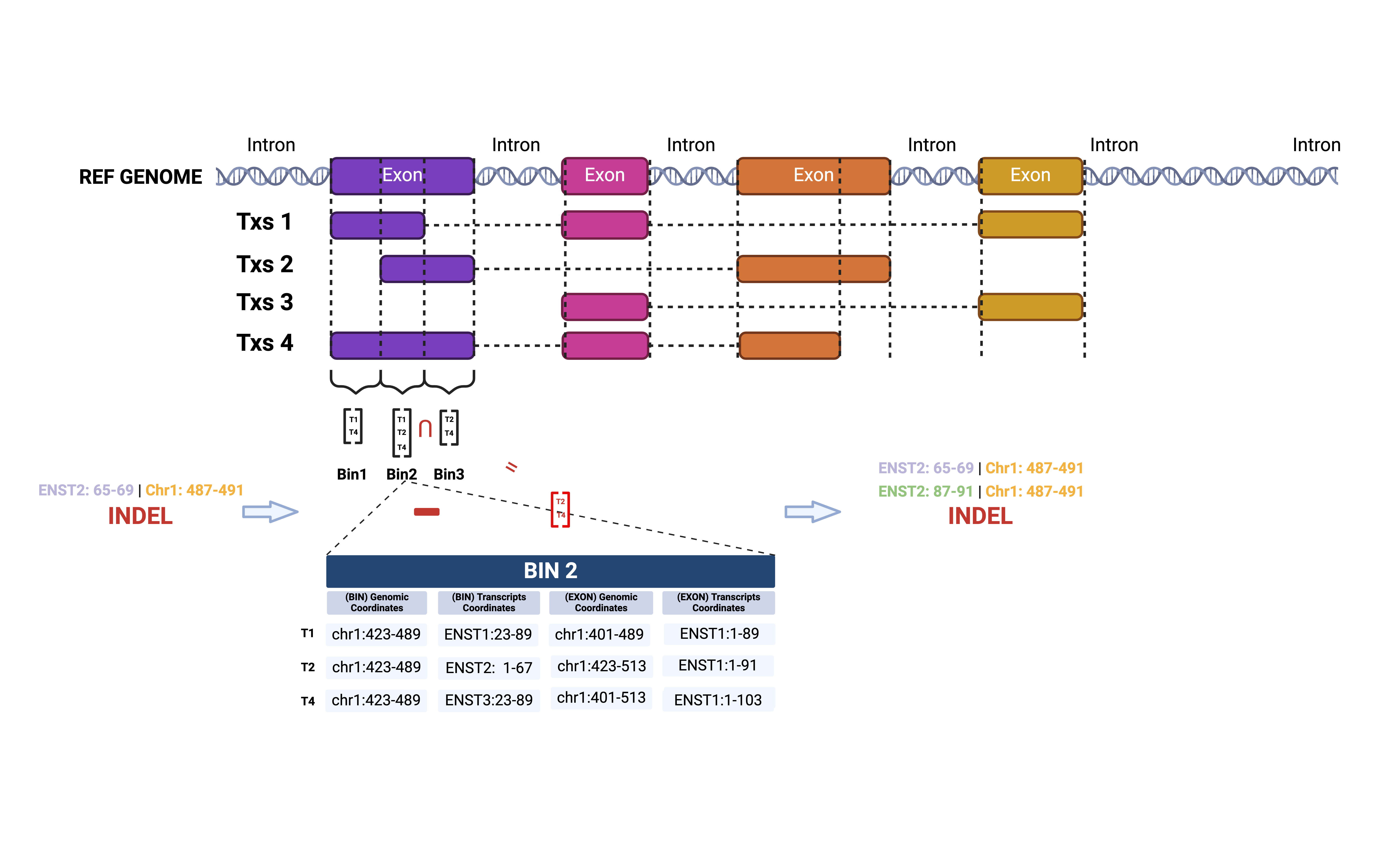
gencode.v36.txs.file = system.file("extdata", "gencode.v36.txs.annotation.subset.gff3",
                             package = "bamSliceR")
getDisjoinOverlapBins(gencode.file.txs = gencode.v36.txs.file) -> gencode.v36.txs.bins

split(gencode.v36.txs.bins$transcript_id, gencode.v36.txs.bins$bin_tag)[1:10]
## $`chr1:226061851-226062094`
## [1] "ENST00000366816.5"
##
## $`chr1:226062714-226062715`
## [1] "ENST00000366814.3"
##
## $`chr1:226062716-226062725`
## [1] "ENST00000366814.3" "ENST00000366815.10"
##
## $`chr1:226062726-226062734`
## [1] "ENST00000366814.3" "ENST00000366815.10" "ENST00000653960.1"
##
## $`chr1:226062735-226062749`
## [1] "ENST00000366816.5" "ENST00000366814.3" "ENST00000366815.10" "ENST00000653960.1"
##
## $`chr1:226062750-226062757`
## [1] "ENST00000366816.5" "ENST00000366814.3" "ENST00000366815.10" "ENST00000653960.1"
## [5] "ENST00000655399.1"
##
## $`chr1:226062758-226062782`
## [1] "ENST00000366816.5" "ENST00000366814.3" "ENST00000366815.10" "ENST00000653960.1"
## [5] "ENST00000655399.1" "ENST00000667897.1"
##
## $`chr1:226062783-226062811`
## [1] "ENST00000366816.5" "ENST00000366814.3" "ENST00000366815.10" "ENST00000653960.1"
## [5] "ENST00000655399.1" "ENST00000667897.1" "ENST00000656829.1"
##
## $`chr1:226062812-226062948`
## [1] "ENST00000655399.1"
##
## $`chr1:226063466-226063493`
## [1] "ENST00000666609.1"fixMissingTxs() would call
getDisjoinOverlapBins() to find all transcripts compatible
with a variant.
oneTxsVariant_file = system.file("extdata", "oneTxsVariant.rds",
                             package = "bamSliceR")
bam.file.dir = system.file("extdata", package = "bamSliceR")
oneTxsVariant = readRDS(oneTxsVariant_file)
oneTxsVariant[,c("UPC_ID", "VAF")]
## VRanges object with 1 range and 2 metadata columns:
## seqnames ranges strand ref alt totalDepth
## <Rle> <IRanges> <Rle> <character> <characterOrRle> <integerOrRle>
## [1] ENST00000343638.9 2590 * C T 72
## refDepth altDepth sampleNames softFilterMatrix | UPC_ID
## <integerOrRle> <integerOrRle> <factorOrRle> <matrix> | <character>
## [1] 63 8 04H138.RNAseq.gencod.. | 04H138
## VAF
## <numeric>
## [1] 0.111111
## -------
## seqinfo: 232117 sequences from gencode.v36.txs genome
## hardFilters: NULL
all_compatible_txs = fixMissingTxs(oneTxsVariant,
                                   gencode.file.txs = gencode.v36.txs.file,
                                   bam.file.dir = bam.file.dir)
all_compatible_txs[,c("UPC_ID", "VAF")]
## VRanges object with 6 ranges and 2 metadata columns:
## seqnames ranges strand ref alt totalDepth
## <Rle> <IRanges> <Rle> <character> <characterOrRle> <integerOrRle>
## [1] ENST00000343638.9 2590 * C T 72
## [2] ENST00000302904.8 2903 * C T 56
## [3] ENST00000436088.6 2708 * C T 71
## [4] ENST00000527034.5 2477 * C T 64
## [5] ENST00000533177.5 2479 * C T 48
## [6] ENST00000393606.7 2672 * C T 0
## refDepth altDepth sampleNames
## <integerOrRle> <integerOrRle> <factorOrRle>
## [1] 63 8 04H138.RNAseq.gencode.v36.minimap2.sorted.bam
## [2] 56 0 04H138.RNAseq.gencode.v36.minimap2.sorted.bam
## [3] 71 0 04H138.RNAseq.gencode.v36.minimap2.sorted.bam
## [4] 64 0 04H138.RNAseq.gencode.v36.minimap2.sorted.bam
## [5] 48 0 04H138.RNAseq.gencode.v36.minimap2.sorted.bam
## [6] 0 0 04H138.RNAseq.gencode.v36.minimap2.sorted.bam
## softFilterMatrix | UPC_ID VAF
## <matrix> | <character> <numeric>
## [1] | 04H138 0.111111
## [2] | 04H138 0.000000
## [3] | 04H138 0.000000
## [4] | 04H138 0.000000
## [5] | 04H138 0.000000
## [6] | 04H138 0.000000
## -------
## seqinfo: 232117 sequences from gencode.v36.txs genome
## hardFilters: NULLAnnotation of Variants
bamSliceR provide wrapper function
getVariantAnnotationForTxs() to annotate Variants by:
- making customized
TxDbobject given thegencode.gff3file - calling
getVariantAnnotation.Txs()&getGenCodeAnnotation.Txs()
- merging annotation results from two sources.
Predict Consequence of Variants
Similar to annotate variants from genomic BAM files, we use
VariantAnnotation to predict consequence of variants in
getVariantAnnotation.Txs().
The only difference is that we need: 1) Create a txdb
object from GENCODE annotation file in GFF3 format that contains
information of both genomic and transcriptome coordinates. 2)
Fasta file contains nucleotide sequences of
transcripts.
# Create txdb object
gencode.v36.txs.file = system.file("extdata", "gencode.v36.txs.annotation.subset.gff3",
                             package = "bamSliceR")
gencode.gr <- import(gencode.v36.txs.file, format="gff3")
metadata = data.frame(name = c("Data source", "Organism","Taxonomy ID", "miRBase build ID"),
                        value= c("GENCODE.v36", "Homo sapiens", "9606", NA))
txdb <- suppressWarnings(makeTxDbFromGRanges(gencode.gr, metadata = metadata))

#getVariantAnnotation.Txs
seqSource = system.file("extdata", "gencode.v36.transcripts.subset.fa",
                        package = "bamSliceR")
leu.tallied.reads.annotated = getVariantAnnotation.Txs(leu.tallied.reads,
                                                       txdb = txdb,
                                                       seqSource = seqSource)
leu.tallied.reads.annotated[3435:3438,c("UPC_ID",bamSliceR:::.VARIANT_ANNOTATE_INFO[1:14])]
## GRanges object with 4 ranges and 15 metadata columns:
## seqnames ranges strand | UPC_ID varAllele CDSLOC
## <Rle> <IRanges> <Rle> | <character> <DNAStringSet> <IRanges>
## [1] ENST00000527034.5 1217 - | 05H195 T 1204
## [2] ENST00000527034.5 1233 - | 05H195 G 1188
## [3] ENST00000527034.5 1335 - | 05H195 T 1086
## [4] ENST00000533177.5 486 - | 05H195 TG 1879
## PROTEINLOC QUERYID TXID CDSID GENEID CONSEQUENCE
## <IntegerList> <integer> <character> <IntegerList> <character> <factor>
## [1] 402 15300 79 488 ENSG00000108312.15 nonsynonymous
## [2] 396 15301 79 488 ENSG00000108312.15 synonymous
## [3] 362 15302 79 489 ENSG00000108312.15 synonymous
## [4] 627 15312 86 531 ENSG00000108312.15 frameshift
## REFCODON VARCODON REFAA VARAA POS CHANGE
## <DNAStringSet> <DNAStringSet> <AAStringSet> <AAStringSet> <integer> <character>
## [1] GAT TAT D Y 402 D402Y
## [2] GGT GGG G G 396 G396G
## [3] CCG CCT P P 362 P362P
## [4] GCC TGCC 627 627
## -------
## seqinfo: 128 sequences from gencode.v36.txs genomeMapping locus with features of Variants.
getGenCodeAnnotation.Txs() will map the locus with
features of variants also from GENCODE annotation file in GFF3 format
that contains information of both genomic and transcriptome coordinates.
But this function not only focus on CDS regions, but also UTR/STOP/START
regions. Further, it will match the transcriptome coordinates of locus
with genomic coordinates.
leu.tallied.reads.gencode = getGenCodeAnnotation.Txs(leu.tallied.reads,
                                                     gencode.file.txs = gencode.v36.txs.file)
leu.tallied.reads.gencode[,c("UPC_ID",bamSliceR:::.GRvsTXS_INFO )]
## VRanges object with 53971 ranges and 11 metadata columns:
## seqnames ranges strand ref alt totalDepth
## <Rle> <IRanges> <Rle> <character> <characterOrRle> <integerOrRle>
## [1] ENST00000366816.5 536-537 * CA C 4
## [2] ENST00000366816.5 578 * C CT 20
## [3] ENST00000366816.5 654 * C CT 11
## [4] ENST00000366816.5 774 * A G 377
## [5] ENST00000366814.3 20 * A C 118
## ... ... ... ... ... ... ...
## [53967] ENST00000358356.9 176 * G GT 6
## [53968] ENST00000358356.9 1433 * A C 22
## [53969] ENST00000358356.9 1439 * G GC 5
## [53970] ENST00000358356.9 1449 * A C 20
## [53971] ENST00000358356.9 1517 * G A 15
## refDepth altDepth sampleNames softFilterMatrix |
## <integerOrRle> <integerOrRle> <factorOrRle> <matrix> |
## [1] 0 4 02H053.RNAseq.gencod.. |
## [2] 0 20 02H053.RNAseq.gencod.. |
## [3] 0 11 02H053.RNAseq.gencod.. |
## [4] 355 19 02H053.RNAseq.gencod.. |
## [5] 112 6 02H053.RNAseq.gencod.. |
## ... ... ... ... ... .
## [53967] 0 6 14H071.RNAseq.gencod.. |
## [53968] 15 4 14H071.RNAseq.gencod.. |
## [53969] 0 5 14H071.RNAseq.gencod.. |
## [53970] 16 4 14H071.RNAseq.gencod.. |
## [53971] 8 7 14H071.RNAseq.gencod.. |
## UPC_ID g_exon_number g_exon_id g_seqid g_start g_end
## <character> <character> <character> <character> <integer> <integer>
## [1] 02H053 4 ENSE00002355903.1 chr1 226065719 226065720
## [2] 02H053 4 ENSE00002355903.1 chr1 226065761 226065761
## [3] 02H053 5 ENSE00001381318.2 chr1 226071378 226071378
## [4] 02H053 5 ENSE00001381318.2 chr1 226071498 226071498
## [5] 02H053 1 ENSE00001442673.3 chr1 226062733 226062733
## ... ... ... ... ... ... ...
## [53967] 14H071 1 ENSE00001380483.1 chr21 34888515 34888515
## [53968] 14H071 1 ENSE00001380483.1 chr21 34887258 34887258
## [53969] 14H071 1 ENSE00001380483.1 chr21 34887252 34887252
## [53970] 14H071 1 ENSE00001380483.1 chr21 34887242 34887242
## [53971] 14H071 1 ENSE00001380483.1 chr21 34887174 34887174
## g_strand g_isCDS g_isSSC gene_name gene_id
## <character> <character> <character> <character> <character>
## [1] + CDS <NA> H3-3A ENSG00000163041.13
## [2] + CDS <NA> H3-3A ENSG00000163041.13
## [3] + CDS <NA> H3-3A ENSG00000163041.13
## [4] + three_prime_UTR <NA> H3-3A ENSG00000163041.13
## [5] + five_prime_UTR <NA> H3-3A ENSG00000163041.13
## ... ... ... ... ... ...
## [53967] - five_prime_UTR <NA> RUNX1 ENSG00000159216.19
## [53968] - five_prime_UTR <NA> RUNX1 ENSG00000159216.19
## [53969] - five_prime_UTR <NA> RUNX1 ENSG00000159216.19
## [53970] - five_prime_UTR <NA> RUNX1 ENSG00000159216.19
## [53971] - five_prime_UTR <NA> RUNX1 ENSG00000159216.19
## -------
## seqinfo: 128 sequences from gencode.v36.txs genome
## hardFilters: NULLMerge annotation results from two sources
In practice, getVariantAnnotationForTxs() can be used to
retrieve annotation results from both sources.
leu.tallied.reads.annoted = getVariantAnnotationForTxs(gencode.file.txs = gencode.v36.txs.file,
                                                       seqSource = seqSource,
                                                       query.ranges = leu.tallied.reads)
head(leu.tallied.reads.annoted)
## GRanges object with 6 ranges and 37 metadata columns:
## seqnames ranges strand | ref alt totalDepth refDepth
## <Rle> <IRanges> <Rle> | <character> <character> <integer> <integer>
## [1] ENST00000366816.5 536-537 * | CA C 4 0
## [2] ENST00000366816.5 578 * | C CT 20 0
## [3] ENST00000366816.5 654 * | C CT 11 0
## [4] ENST00000366816.5 774 * | A G 377 355
## [5] ENST00000366814.3 20 * | A C 118 112
## [6] ENST00000366814.3 97 * | G GGGTA 13 0
## altDepth VAF sample file_name case_id
## <integer> <numeric> <character> <character> <character>
## [1] 4 1.0000000 02H053 02H053.RNAseq.gencod.. 02H053
## [2] 20 1.0000000 02H053 02H053.RNAseq.gencod.. 02H053
## [3] 11 1.0000000 02H053 02H053.RNAseq.gencod.. 02H053
## [4] 19 0.0503979 02H053 02H053.RNAseq.gencod.. 02H053
## [5] 6 0.0508475 02H053 02H053.RNAseq.gencod.. 02H053
## [6] 13 1.0000000 02H053 02H053.RNAseq.gencod.. 02H053
## sample_type experimental_strategy downloaded_file_name UPC_ID
## <character> <character> <character> <character>
## [1] Bone marrow_Diagnosis RNA-Seq STAR 2-Pass .. 02H053.RNAseq.gencod.. 02H053
## [2] Bone marrow_Diagnosis RNA-Seq STAR 2-Pass .. 02H053.RNAseq.gencod.. 02H053
## [3] Bone marrow_Diagnosis RNA-Seq STAR 2-Pass .. 02H053.RNAseq.gencod.. 02H053
## [4] Bone marrow_Diagnosis RNA-Seq STAR 2-Pass .. 02H053.RNAseq.gencod.. 02H053
## [5] Bone marrow_Diagnosis RNA-Seq STAR 2-Pass .. 02H053.RNAseq.gencod.. 02H053
## [6] Bone marrow_Diagnosis RNA-Seq STAR 2-Pass .. 02H053.RNAseq.gencod.. 02H053
## varAllele CDSLOC PROTEINLOC QUERYID TXID CDSID
## <DNAStringSet> <IRanges> <IntegerList> <integer> <character> <IntegerList>
## [1] C 192-193 64,65 1 22 212
## [2] CT 234 78 2 22 212
## [3] CT 310 104 3 22 213
## [4] N -1 <NA> <NA> <NA> <NA>
## [5] N -1 <NA> <NA> <NA> <NA>
## [6] N -1 <NA> <NA> <NA> <NA>
## GENEID CONSEQUENCE REFCODON VARCODON REFAA
## <character> <character> <DNAStringSet> <DNAStringSet> <AAStringSet>
## [1] ENSG00000163041.13 frameshift CGCAAA CGCAA
## [2] ENSG00000163041.13 frameshift GAC GACT
## [3] ENSG00000163041.13 frameshift CTT CTTT
## [4] ENSG00000163041.13 <NA> N N N
## [5] ENSG00000163041.13 <NA> N N N
## [6] ENSG00000163041.13 <NA> N N N
## VARAA POS CHANGE SYMBOL HGVSP g_exon_number
## <AAStringSet> <integer> <character> <character> <character> <character>
## [1] 64 64 H3-3A H3-3A64 4
## [2] 78 78 H3-3A H3-3A78 4
## [3] 104 104 H3-3A H3-3A104 5
## [4] N <NA> <NA> H3-3A <NA> 5
## [5] N <NA> <NA> H3-3A <NA> 1
## [6] N <NA> <NA> H3-3A <NA> 1
## g_exon_id g_seqid g_start g_end g_strand g_isCDS
## <character> <character> <integer> <integer> <character> <character>
## [1] ENSE00002355903.1 chr1 226065719 226065720 + CDS
## [2] ENSE00002355903.1 chr1 226065761 226065761 + CDS
## [3] ENSE00001381318.2 chr1 226071378 226071378 + CDS
## [4] ENSE00001381318.2 chr1 226071498 226071498 + three_prime_UTR
## [5] ENSE00001442673.3 chr1 226062733 226062733 + five_prime_UTR
## [6] ENSE00001442673.3 chr1 226062810 226062810 + five_prime_UTR
## g_isSSC
## <character>
## [1] <NA>
## [2] <NA>
## [3] <NA>
## [4] <NA>
## [5] <NA>
## [6] <NA>
## -------
## seqinfo: 128 sequences from gencode.v36.txs genomeUsing Genomic VAF as Prior to Infer Transcripts’ VAF
![]()
We now have both Genomic and Transcriptome annotation for each variants. Specifically, We know the ref and alt read counts and VAF from genomic alignment that mapped reads to the linear reference genome. We also have such information for each transcripts of the gene by mapping reads against transcripts’ sequences. Now, the question is how can we infer which transcript carried the variants being expressed based on the reads mapping evidence.
Rather than pretending that all of the evidence has equal weight, we instead can test for the null that each compatible transcript has a VAF generated from the same underlying distribution sampled by genomic VAF of variant (g_VAF) with total_depth trials. Then our prior would be Pr(variant on transcript X) == Pr(variant on gDNA), when g_VAF follows Beta distribution Beta(g_depth_ref, g_depth_alt).
For example:
#contains all recurrent variants that compatible with more than one transcripts
gVSt_file = system.file("extdata", "GvsT_recurrent_multiTxs_list.rds",
                             package = "bamSliceR")
GvsT_recurrent_multiTxs_list = readRDS(gVSt_file)

#one patient one variant
demo = GvsT_recurrent_multiTxs_list[[16]][1:4,]
demo
## DataFrame with 4 rows and 32 columns
## g_seqid g_start g_end strand g_UPC_ID g_ref g_alt
## <character> <integer> <integer> <factor> <character> <character> <character>
## 1 chr15 90085321 90085321 * 02H060 T C
## 2 chr15 90085321 90085321 * 02H060 T C
## 3 chr15 90085321 90085321 * 02H060 T C
## 4 chr15 90085321 90085321 * 02H060 T C
## g_totalDepth g_refDepth g_altDepth g_VAF t_gseqid t_gstart t_gend
## <numeric> <numeric> <integer> <numeric> <character> <integer> <integer>
## 1 1013 911 98 0.0967423 chr15 90085321 90085321
## 2 1013 911 98 0.0967423 chr15 90085321 90085321
## 3 1013 911 98 0.0967423 chr15 90085321 90085321
## 4 1013 911 98 0.0967423 chr15 90085321 90085321
## t_UPC_ID t_ref t_alt t_totalDepth t_refDepth t_altDepth t_VAF
## <character> <character> <character> <numeric> <numeric> <integer> <numeric>
## 1 02H060 T C 258 248 10 0.0387597
## 2 02H060 T C 228 212 16 0.0701754
## 3 02H060 T C 221 209 11 0.0497738
## 4 02H060 T C 223 204 19 0.0852018
## t_tseqid t_tstart t_tend SYMBOL CHANGE g_len t_len
## <character> <integer> <integer> <character> <character> <integer> <integer>
## 1 ENST00000330062.8 1112 1112 IDH2 E345G 1 1
## 2 ENST00000560061.1 854 854 IDH2 NA 1 1
## 3 ENST00000559482.5 794 794 IDH2 E236G 1 1
## 4 ENST00000540499.2 1039 1039 IDH2 E293G 1 1
## min_start max_end DNAstring variant_tag
## <integer> <integer> <DNAStringSet> <character>
## 1 90085321 90085321 T chr15:90085321:90085..
## 2 90085321 90085321 T chr15:90085321:90085..
## 3 90085321 90085321 T chr15:90085321:90085..
## 4 90085321 90085321 T chr15:90085321:90085..
plotHistAsDist = function(data, binwidth = 0.001, i)
{
  data = data.frame(d = 1:nrow(data), average = data[,i])
  ggplot(data, aes(x = average)) +
    geom_histogram(binwidth = binwidth, fill = "blue", color = "black", alpha = 0.7) +
    labs(title = "Distribution of True Averages",
         x = "True Average",
         y = "Frequency") +
    theme_minimal()
}

#Example:V = "chr15:90085321:90085321:T:C" patient:"02H060"
#g_VAF = 0.0967423
#g_altDepth = 98
#g_refDepth = 911
#EC:"ENST00000330062.8", "ENST00000560061.1", "ENST00000559482.5", "ENST00000540499.2"

#model 1: VAF(ENST00000330062.8) == g_VAF(V)
#t_totalDepth(ENST00000330062.8) == 258
#t_altDepth(ENST00000330062.8) == 10
#t_refDepth(ENST00000330062.8) == 248
#1) assume that in model 1 the prior distribution for theta(VAF)
# is Beta(g_altDepth, g_refDepth) == Beta(98, 911)
# The observed data for "ENST00000330062.8" tells us that there
# are 258 "bernoulli trails"(txs total depth), and 10 "success" (txs alt depth).

#Use simulation to approximate the probability of observing 10 "success"
#in 258 "bernoulli trails" given that model 1 is correct.

Nrep = 1000000
g_VAF = rbeta(Nrep, 98, 911)
theta_df = data.frame(theta = g_VAF, no = 1:length(g_VAF))
plotHistAsDist(theta_df,
               binwidth = 0.001,
               i = which(colnames(theta_df) == "theta"))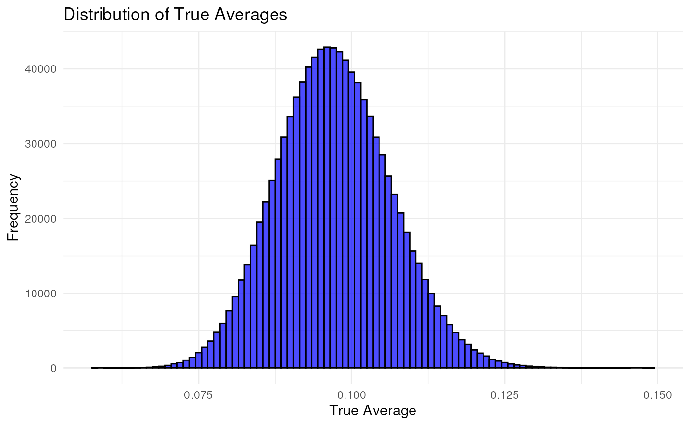
## [1] 0.000636We can do Bayesian model comparison to calculate Bayes factor from these two models: model 1: Pr(V|Tx in TxCanHarborV) == Pr(V) for all Tx in TxCanHarborV (prior for Pr(V) is Pr(V|gDNA)) model 2: Pr(V|Tx in TxCanHarborV) != Pr(V) for all Tx in TxCanHarborV (prior as above)
Example of integrating over the parameter space for the possible evidence:
## Approximation of integrate over the parameter space for the possible evidence
theta = seq(0,1,0.00001)
#p(theta|M) = p(g_VAF|beta dist)
prior_of_theta = dbeta(theta, 98, 911)

#likelihood p(X | theta) == p(alt_txs_reads | g_VAF)
likelihood = dbinom(10 , 258, theta)

# integral of p(X| theta, M) * p(theta | M) dtheta
mg_txs1 = sum(likelihood * prior_of_theta * theta)
Extract reads from BAM files for variants
## Approximation of integrate over the parameter space for the possible evidence
theta = seq(0,1,0.00001)
#p(theta|M) = p(g_VAF|beta dist)
prior_of_theta = dbeta(theta, 98, 911)

#likelihood p(X | theta) == p(alt_txs_reads | g_VAF)
likelihood = dbinom(10 , 258, theta)

# integral of p(X| theta, M) * p(theta | M) dtheta
mg_txs1 = sum(likelihood * prior_of_theta * theta)
For any given transcript, the universe of reads supporting it may or may not overlap with the others. The degree to which this is the case determines how correlated (or not) the results of the tests are expected to be.
In bamSliceR we provide function
extractBasesAtPosition() to collect read names support
either reference or alternative alleles for on each transcripts.
#one patient one variant
demo[1,c("t_totalDepth", "t_refDepth", "t_altDepth", "t_VAF", "t_tseqid", "SYMBOL", "CHANGE")]
## DataFrame with 1 row and 7 columns
## t_totalDepth t_refDepth t_altDepth t_VAF t_tseqid SYMBOL CHANGE
## <numeric> <numeric> <integer> <numeric> <character> <character> <character>
## 1 258 248 10 0.0387597 ENST00000330062.8 IDH2 E345G
genomicPosition = GRanges(seqnames = demo$t_tseqid[1],
                          ranges = IRanges(start = demo$t_tstart[1], end = demo$t_tend[1]) )
bamFile = system.file("extdata","02H060.RNAseq.gencode.v36.minimap2.sorted.bam",
                              package = "bamSliceR")
readsPerTxs = extractBasesAtPosition(bamFile = bamFile, which = genomicPosition)
table(readsPerTxs[[1]])
##
## A G N
## 248 10 19## R version 4.4.1 (2024-06-14)
## Platform: x86_64-pc-linux-gnu
## Running under: Ubuntu 22.04.4 LTS
##
## Matrix products: default
## BLAS: /usr/lib/x86_64-linux-gnu/openblas-pthread/libblas.so.3
## LAPACK: /usr/lib/x86_64-linux-gnu/openblas-pthread/libopenblasp-r0.3.20.so; LAPACK version 3.10.0
##
## locale:
## [1] LC_CTYPE=en_US.UTF-8 LC_NUMERIC=C LC_TIME=en_US.UTF-8
## [4] LC_COLLATE=en_US.UTF-8 LC_MONETARY=en_US.UTF-8 LC_MESSAGES=en_US.UTF-8
## [7] LC_PAPER=en_US.UTF-8 LC_NAME=C LC_ADDRESS=C
## [10] LC_TELEPHONE=C LC_MEASUREMENT=en_US.UTF-8 LC_IDENTIFICATION=C
##
## time zone: Etc/UTC
## tzcode source: system (glibc)
##
## attached base packages:
## [1] parallel stats4 stats graphics grDevices utils datasets methods
## [9] base
##
## other attached packages:
## [1] Homo.sapiens_1.3.1 TxDb.Hsapiens.UCSC.hg19.knownGene_3.2.2
## [3] org.Hs.eg.db_3.19.1 GO.db_3.19.1
## [5] OrganismDbi_1.47.0 GenomicFeatures_1.57.0
## [7] AnnotationDbi_1.67.0 ggplot2_3.5.1
## [9] rtracklayer_1.65.0 bamSliceR_0.1.2
## [11] GenomicDataCommons_1.29.3 plyranges_1.25.0
## [13] VariantAnnotation_1.51.0 SummarizedExperiment_1.35.1
## [15] Biobase_2.65.0 MatrixGenerics_1.17.0
## [17] matrixStats_1.3.0 gmapR_1.47.0
## [19] Rsamtools_2.21.0 Biostrings_2.73.1
## [21] XVector_0.45.0 GenomicRanges_1.57.1
## [23] GenomeInfoDb_1.41.1 IRanges_2.39.2
## [25] S4Vectors_0.43.2 BiocGenerics_0.51.0
##
## loaded via a namespace (and not attached):
## [1] RColorBrewer_1.1-3 jsonlite_1.8.8
## [3] magrittr_2.0.3 farver_2.1.2
## [5] rmarkdown_2.27 fs_1.6.4
## [7] BiocIO_1.15.0 zlibbioc_1.51.1
## [9] ragg_1.3.2 vctrs_0.6.5
## [11] memoise_2.0.1 RCurl_1.98-1.16
## [13] htmltools_0.5.8.1 S4Arrays_1.5.5
## [15] progress_1.2.3 curl_5.2.1
## [17] SparseArray_1.5.25 sass_0.4.9
## [19] bslib_0.7.0 htmlwidgets_1.6.4
## [21] desc_1.4.3 httr2_1.0.2
## [23] cachem_1.1.0 GenomicAlignments_1.41.0
## [25] lifecycle_1.0.4 pkgconfig_2.0.3
## [27] Matrix_1.7-0 R6_2.5.1
## [29] fastmap_1.2.0 GenomeInfoDbData_1.2.12
## [31] digest_0.6.36 colorspace_2.1-0
## [33] maftools_2.21.0 textshaping_0.4.0
## [35] RSQLite_2.3.7 labeling_0.4.3
## [37] filelock_1.0.3 fansi_1.0.6
## [39] httr_1.4.7 abind_1.4-5
## [41] compiler_4.4.1 bit64_4.0.5
## [43] withr_3.0.0 BiocParallel_1.39.0
## [45] DBI_1.2.3 highr_0.11
## [47] biomaRt_2.61.2 rappdirs_0.3.3
## [49] DelayedArray_0.31.9 rjson_0.2.21
## [51] DNAcopy_1.79.0 tools_4.4.1
## [53] glue_1.7.0 restfulr_0.0.15
## [55] VariantTools_1.47.0 grid_4.4.1
## [57] generics_0.1.3 gtable_0.3.5
## [59] BSgenome_1.73.0 tzdb_0.4.0
## [61] data.table_1.15.4 hms_1.1.3
## [63] xml2_1.3.6 utf8_1.2.4
## [65] pillar_1.9.0 stringr_1.5.1
## [67] splines_4.4.1 dplyr_1.1.4
## [69] BiocFileCache_2.13.0 lattice_0.22-6
## [71] survival_3.7-0 bit_4.0.5
## [73] tidyselect_1.2.1 BSgenome.Hsapiens.UCSC.hg38_1.4.5
## [75] RBGL_1.81.0 knitr_1.48
## [77] xfun_0.46 stringi_1.8.4
## [79] UCSC.utils_1.1.0 yaml_2.3.9
## [81] TxDb.Hsapiens.UCSC.hg38.knownGene_3.18.0 evaluate_0.24.0
## [83] codetools_0.2-20 tibble_3.2.1
## [85] BiocManager_1.30.23 graph_1.83.0
## [87] cli_3.6.3 systemfonts_1.1.0
## [89] munsell_0.5.1 jquerylib_0.1.4
## [91] dbplyr_2.5.0 png_0.1-8
## [93] XML_3.99-0.17 pkgdown_2.1.0
## [95] readr_2.1.5 blob_1.2.4
## [97] prettyunits_1.2.0 bitops_1.0-7
## [99] txdbmaker_1.1.1 scales_1.3.0
## [101] purrr_1.0.2 crayon_1.5.3
## [103] rlang_1.1.4 KEGGREST_1.45.1